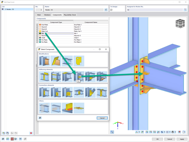
Mit der Komponente "Rippe" können Sie sehr schnell eine beliebige Anzahl an Längsrippen an einem Stabblech definieren. Durch die Vorgabe eines Referenzobjektes lassen sich daran automatisch Schweißnähte vorgeben.
Die Komponente "Rippe" lässt sich auch an kreisförmigen Hohlprofilen anordnen. Dafür wird zusätzlich die Vorgabe der Winkel zwischen den Rippen benötigt.
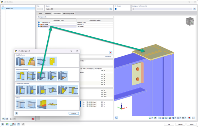
You can now insert a cap plate in steel joints with only a few clicks. You can enter the data using the known definition types "Offsets" or "Dimensions and Position". By specifying a reference member and the cutting plane, it is also possible to omit the Member Section component.
This component allows you to easily model cap plates on column ends, for example.
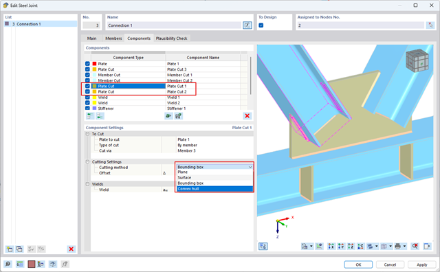
You can use the "Plate Cut" component to cut plates (for example, gusset plates, fin plates, and so on). There are various cutting methods available:
- Plane: The cut is performed on the closest surface to the reference plate.
- Surface: Only the intersecting parts of plates are cut.
- Bounding Box: The outermost dimension consisting of width and height is cut out of the plate as a rectangle.
- Convex Envelope: The outer hull of the cross-section is used for the plate cut. If there are fillets at the corner nodes of the cross-section, the cut is adapted to them.
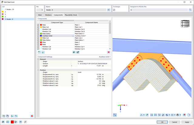
In the Steel Joints add-on, you can perform precise cuts on plates and structural components using the "Auxiliary Solid" component. Within this component, you can use the shapes of a box, a cylinder, or any cross-section as a guide object.
Go to Explanatory Video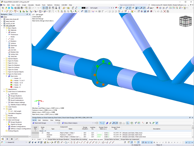
The Steel Joints add-on provides you with the option to connect circular hollow sections using welds.
It is possible to connect the circular sections to each other or to planar structural components. The fillets of standard and thin-walled sections can also be connected with a weld.
Go to Explanatory Video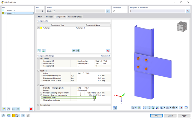
In the Steel Joints add-on, you have this option to consider the preloaded bolts in the calculation of all components.
You can easily activate the prestress using the check box in the bolt parameters, and it has an impact on the stress-strain analysis as well as the stiffness analysis.
Go to Explanatory Video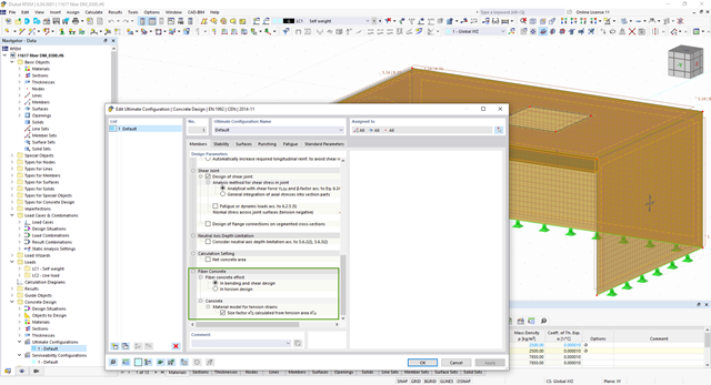
The Concrete Design add-on allows you to design fiber-reinforced concrete components according to the guideline "DAfStb Steel Fiber-Reinforced Concrete".
You can use this option for the design according to EN 1992‑1‑1. The design according to the DAfStb guideline is carried out once the concrete of the "Fiber Concrete" type has been assigned to the reinforced structural component.
Go to Explanatory Video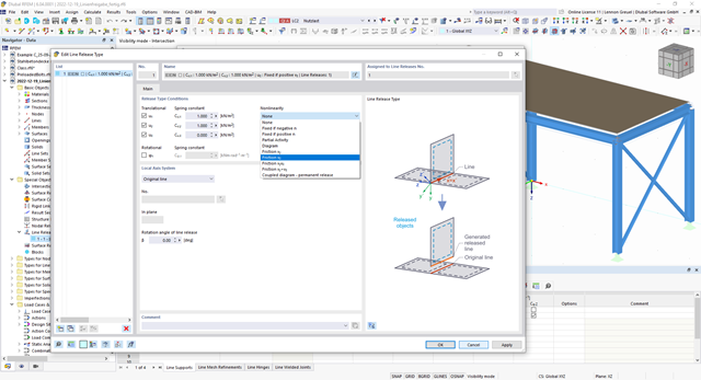
You can simulate the static friction effects between two supporting components along a line using the "Friction" nonlinearity in the Line Release Type.
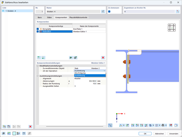
In the Member Editor component, you can also select the entire member as the modifying object instead of the individual member plates. This way, you can apply both operations "Notch" and "Chamfer" to several member plates.

Using the "Load Transfer Only" story type, you can consider slabs without stiffness effect in and out of the plane in the Building Model add-on. This element type collects the loads on the slab and transfers them to the supporting elements of a 3D model. Thus, you can simulate secondary components, such as grillage and similar load distribution elements, without any further effect in the 3D model.
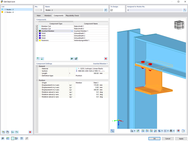
When designing connections, you can now also insert a new member as a component directly in the Steel Joints add-on. This will only be considered for the connection design. You can use the Weld and Fasteners components to connect to other members.
Furthermore, it is possible to use the Member Section and Member Editor components and arrange reinforcement elements on the inserted member, such as stiffeners and tapers.
Go to Explanatory Video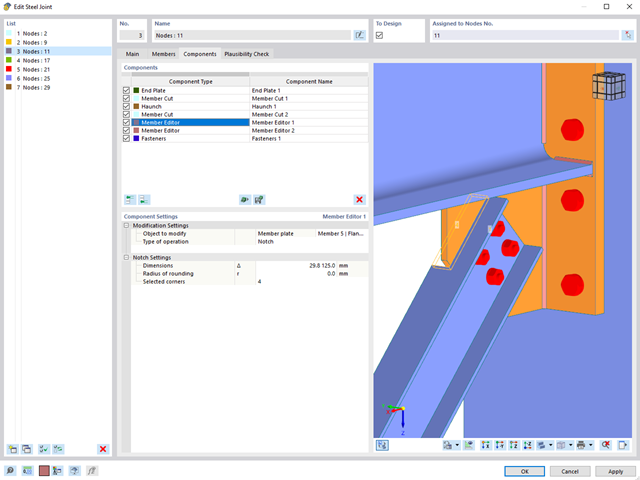
The "Member Editor" component allows you to modify the individual or several member plates in the Steel Joints add-on.
You can use the chamfer, notch, rounding, and hole operations with multiple shapes. It is possible to apply both operations, "Notch" and "Chamfer", for several member plates.
In this way, you can notch flanges from I-sections, for example (see the image).
Go to Explanatory Video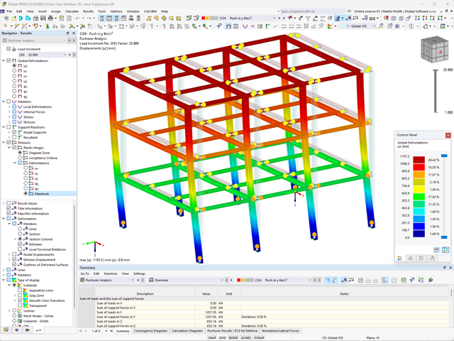
- Consideration of nonlinear component behavior using plastic standard hinges for steel (FEMA 356, EN 1998‑3) and nonlinear material behavior (masonry, steel - bilinear, user-defined working curves)
- Direct import of masses from load cases or combinations for the application of constant vertical loads
- User-defined specifications for the consideration of horizontal loads (standardized to a mode shape or uniformly distributed over the height of the masses)
- Determination of a pushover curve with selectable limit criterion of the calculation (a collapse or limit deformation)
- Transformation of the pushover curve into the capacity spectrum (ADRS format, single degree of freedom system)
- Bilinearization of the capacity spectrum according to EN 1998‑1:2010 + A1:2013
- Transformation of the applied response spectrum into the required spectrum (ADRS format)
- Determination of target displacement according to EC 8 (the N2 method according to Fajfar 2000)
- Graphical comparison of the capacity and required spectrum
- Graphical evaluation of the acceptance criteria of predefined plastic hinges
- Result display of the values used in the iterative calculation of the target displacement
- Access to all results of the structural analysis in the individual load levels
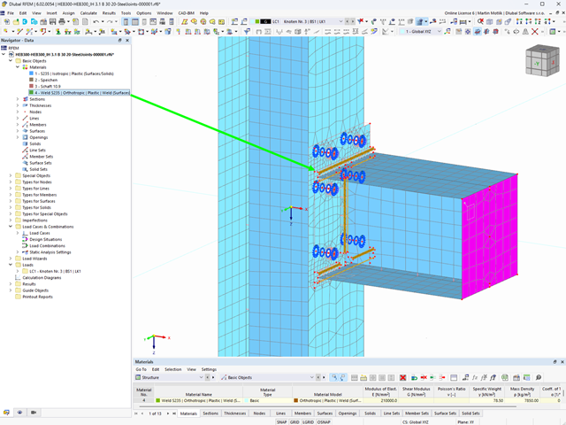
Here, the weld design becomes child's play. Using the specially developed material model "Orthotropic | Plastic | Weld (Surfaces)", you can calculate all stress components plastically. The stress τperpendicular is also considered plastically.
Using this material model you can design welds closer to reality and more efficiently.
Go to Explanatory Video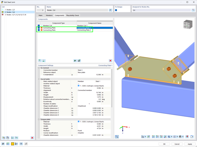
Using the "Connecting Plate" component, you can additionally and automatically create a new gusset plate in the Steel Joints add-on. This saves you separate components, and the other elements, such as a cap plate and a slide plate, are thus automatically taken into account with their dimensions.
Go to Explanatory Video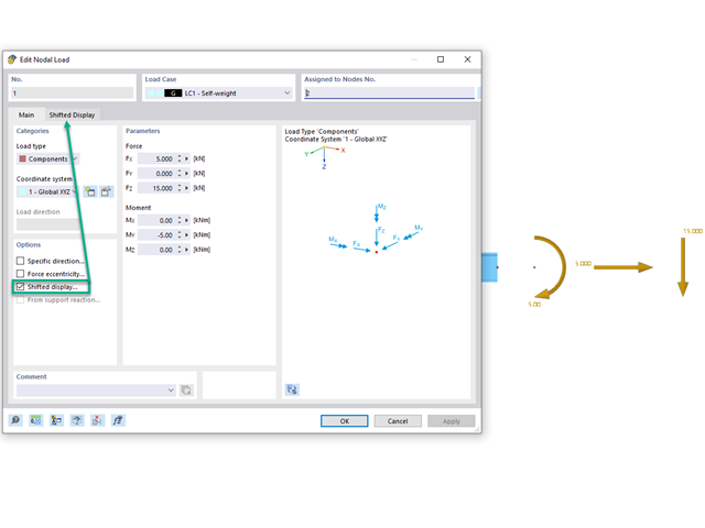
Would you like to display nodal loads or load components that act on one point next to each other? Then use the "Shifted Display" option. This allows you to define offsets in the x, y, and z directions, as well as the size and spacing.
Go to Explanatory Video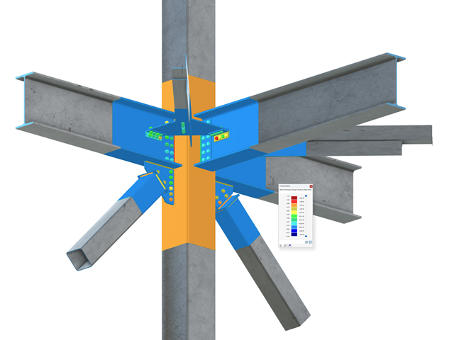
Complex Connection of Horizontal Beams to Column and Connection of Reinforcing Diagonals
The connection model was modeled using about 50 components. The model was created according to the real example of use in structure.
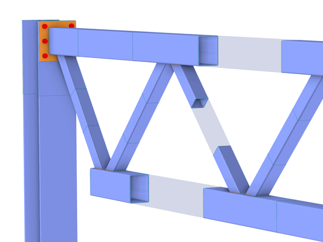
In the case of rectangular cross-sections, you can usually achieve a direct connection by using welds. However, you can also connect them to other cross-sections in the same way. Furthermore, other components such as end plates help you to connect the rectangular cross-sections to other structural components.
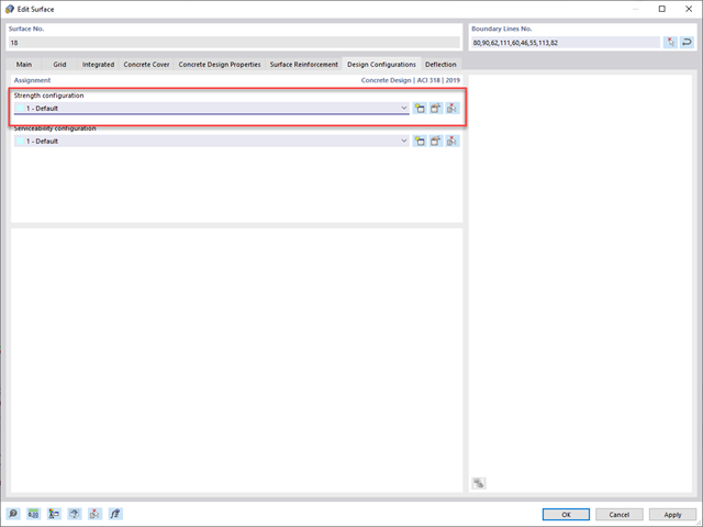
Do you work with the structural components consisting of slabs? In that case, you have to perform the shear force design with the requirements of punching shear design, for example, according to 6.4, EN 1992‑1‑1. In addition to floor slabs, you can also design foundation slabs in this way.
In the Ultimate Configuration for concrete design, you can define the punching design parameters for the selected nodes.
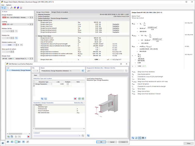
You know for sure that when connecting tension-loaded components with bolted connections, you need to consider the cross-section reduction due to the bolt holes in the ultimate limit state design. The structural analysis programs also have a solution for this. In the Aluminum Design add-on, you can enter a member local section reduction for this. Enter the reduction of the cross-section as an absolute value or as a percentage of the total area at all relevant locations.
You already know that it is possible to model and analyze a soil and a structure in the entire model. As a result, you have explicitly taken into account the soil-structure interaction. By modifying a component, you achieve the immediate correct consideration in the analysis as well as in the results for the entire system of the soil and structure.
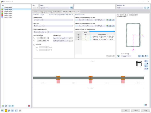
The program does a lot of work for you. For example, the load or result combinations required for the serviceability limit state are generated and calculated in RFEM/RSTAB. You can select these design situations for the deflection analysis in the Aluminum Design add-on. Depending on the specified precamber and reference system, the program determines the deformation values at each location of a member. They are then compared to the limit values.
You can specify the deformation limit value individually for each structural component in Serviceability Configuration. In this case, you define the maximum deformation depending on the reference length as the allowable limit value. By defining design supports, you can segment the components. In this way, you can determine the corresponding reference length automatically for each design direction.
And that's not all. Based on the position of the assigned design supports, the program allows you to automatically determine the distinction between beams and cantilevers. The limit value is thus determined accordingly.

As you've already learned, the results of a Modal Analysis load case are displayed in the program after a successful calculation. You can thus immediately see the first mode shape graphically or as an animation. You can also easily adjust the representation of the mode shape standardization. Do that directly in the Results navigator, where you have one of four options for the visualization of the mode shapes available for the selection:
- Scaling the value of the mode shape vector uj to 1 (considers the translation components only)
- Selecting the maximum translational component of the eigenvector and setting it to 1
- Considering the entire eigenvector (including the rotation components), selecting the maximum, and setting it to 1
- Setting the modal mass mi for each mode shape to 1 kg
You can find a detailed explanation of the mode shape standardization in the OnlineManual here.
The deformation process of the global deformation components can be represented as a movement sequence.
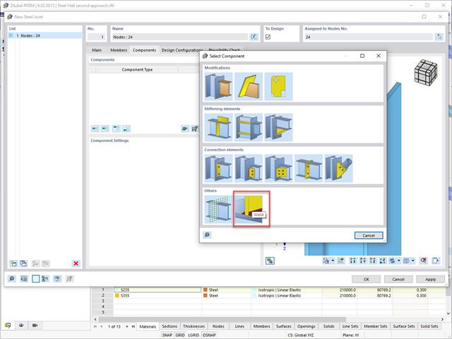
In addition to other predefined components in the design add-on for steel connections, the universal base component "General Weld" can be used to enter complex connection situations.

Do you want to consider other loads as masses in addition to the static loads? The program allows that for nodal, member, line and surface loads. For this, you need to select the Mass load type when defining the load of interest. Define a mass or mass components in the X, Y, and Z directions for such loads. For nodal masses, you have an additional option to also specify moments of inertia X, Y, and Z in order to model more complex mass points.

It is often necessary to neglect masses. This is particularly the case when you want to use the output of the modal analysis for the seismic analysis. For this, 90% of the effective modal mass in each direction is required for the calculation. So you can neglect the mass in all fixed nodal and line supports. The program automatically deactivates the associated masses for you.
You can also manually select the objects whose masses are to be neglected for the modal analysis. We have shown the latter in the image for a better view. A user-defined selection is made the and the objects with their associated mass components are selected to neglect the masses.

You have several options available to define masses for a modal analysis. While the masses due to self-weight are considered automatically, you can consider the loads and masses directly in a load case of the modal analysis type. Do you need more options? Select whether to consider full loads as masses, load components in the global Z-direction, or only the load components in the direction of gravity.
The program offers you an additional or alternative option for importing masses: A manual definition of load combinations as of which are the masses considered in the modal analysis. Have you selected a design standard? You can then create a design situation with the Seismic Mass combination type. Thus, the program automatically calculates a mass situation for the modal analysis according to the preferred design standard. In other words: The program creates a load combination on the basis of the preset combination coefficients for the selected standard. This contains the masses used for the modal analysis.
- The design of the connection components is performed according to AISC 360-16 and Eurocode EN 1993-1-8
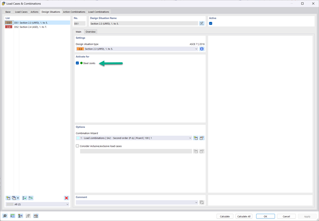
- After activating the Add-on, the design situations for Steel Connections must be activated in the 'Load cases and Combinations' dialog box
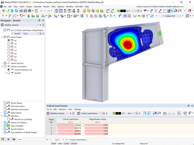
- For the design of the connection stability (Buckling), it is necessary to have the Add-on Structure Stability activated
- The calculation can be started via the table or via the icon in the top bar
- The steel connections model and the results can be saved as a separate model file
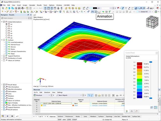
- The resulting stresses and the results of the stability analysis (joint buckling) can be displayed in a separate model
- In the saved model, you can run a deformation animation on the connection
- Connection components are converted to surfaces and members when they are saved